Forecasting the COVID-19 Pandemic Evolution in Queretaro
Summary
This is a research project, carried out with Dr. U. Velasco and Eng. B. Salgado, that aims to estimate the maximum number of infected people and mortality rate due to the Covid-19 pandemic in Queretaro. The SIR model was used in conjunction with the 4th order Runge-Kutta method to numerically solve the system.

Date
- Data Science
Category
Python
Tools
A New Virus, a World in Mourning
What began as a quarantine has turned into over half a year of waiting for things to improve. Despite the efforts of health authorities, as of November 14, 2020, there have been over 100,000 COVID-19 deaths in Mexico alone, and there’s no sign that the number will stop rising anytime soon.

This pandemic has not only affected our health and economy, but also our entire way of life. For this reason, we find it necessary to conduct this study to estimate the future impact of the pandemic (in the state of Querétaro, our home).
Workflow
The development of this project was divided into 5 phases:
Theoretical Framework
Research was conducted on the SIR model and the 4th order Runge-Kutta model. The objectives of the research project were defined.
Kermack-Mckendrick (SIR) Model for the Spread of Viral Infections
Kermack-Mckendrick (SIR) Model for the Spread of Viral Infections
In the SIR model, the objective is to determine what proportion of the total population will be infected and for how long.
We begin the formulation of the model by dividing the population into three subclasses that will be designated with the letters S, I and R. Firstly, S(t) will denote the number of individuals susceptible to contracting the disease at time t, I(t) the number of individuals capable of transmitting it; that is, infectious individuals, and R(t) the number of recovered or deceased individuals in the population at time t. [1].
The model is presented as a coupled system of equations as follows:
[math]\frac{dS}{dt} = -\beta SI [/math]
[math]\frac{dI}{dt} = \beta SI – \gamma I [/math]
[math]\frac{dR}{dt} = \gamma I [/math]
Where,
- [math]\frac{dS}{dt}, \frac{dI}{dt}, \frac{dR}{dt}[/math] are the functions that describe how the number of individuals in the susceptible, infected and recovered groups changes over time t.
[math]\beta[/math] is the rate of disease transmission. It represents the probability that a susceptible individual will become infected by coming into contact with an infected individual.
[math]\gamma[/math] is the recovery rate. It represents the fraction of infected individuals that recover per unit of time.
Also, this model is based on the following assumptions:
- All deaths are caused by the disease.
- The rate of new infections is proportional to the total number of contacts between susceptible and infected individuals (beta).
- The recovery rate of infected individuals is constant (gamma).
- During the course of the epidemic the net birth rate is zero.
The SIR model has no analytical solutions, but we can use numerical methods to approximate the solution to the model with great precision.
Fourth Order Runge-Kutta Method
Fourth Order Runge-Kutta Method
The 4th order Runge-Kutta method (RK4) is a numerical method used to solve ordinary differential equations (ODEs) with an initial value. In essence, Runge-Kutta methods are generalizations of Euler’s basic formula, in which the slope function is replaced by a weighted average of slopes ([math]k_1, … k_4[/math]) in the interval x with step size [math]h[/math]. [3]
This model proposes to find certain parameters w that must meet a series of conditions that we will not explain in detail. Instead, we will show the most frequently used set of values for the parameters w:
[math]y_{n+1} = y_n + \frac{h}{6} (k_1 + 2k_2 + 2k_3 + k_4)[/math]
where,
[math]k_1 = f(x_n, y_n)[/math]
[math]k_2 = f(x_n + \frac{h}{2}, y_n + \frac{h}{2} k_1)[/math]
[math]k_3 = f(x_n + \frac{h}{2}, y_n + \frac{h}{2} k_2)[/math]
[math]k_4 = f(x_n + h, y_n + h k_3)[/math]
And [math]f(x_n, y_n)[/math] is the differential function we are trying to solve. In our case, these would be the expressions for [math]\frac{dS}{dt}[/math], [math]\frac{dI}{dt}[/math], and [math]\frac{dR}{dt}[/math].
This method has an error of order [math]h^4[/math]. [3]
Finite Difference Method
Finite Difference Method
The derivative expression for a function F(x) is defined by,
[math]F'(x) = \lim_{\Delta x \rightarrow 0} \frac{F(x + \Delta x) – F(x)}{\Delta x}[/math]
If we make [math]\Delta x[/math] not tend to zero, but be a small value, we obtain that
[math]F'(x) \approx \frac{F(x + \Delta x) – F(x)}{\Delta x} + O(h)[/math]
Where [math]O(h)[/math] represents an error of order h (result of not having taken the limit when [math]x \rightarrow 0[/math]). [4]
Estimating Beta and Gamma Using Finite Differences
Estimating Beta and Gamma Using Finite Differences
Beta (Transmission Rate): The transmission rate [math]\beta[/math] represents how often susceptible individuals become infected. Using finite differences, we can estimate [math]\beta[/math] from the change in the number of susceptibles (S) and infected (I) individuals over a time interval [math]\Delta t[/math]
From the susceptible equation:
[math]\frac{dS}{dt} = -\beta SI [/math]
We can approximate this as:
[math]\beta \approx \frac{S(t) – S(t + \Delta t)}{S(t) * I(t) * \Delta t}[/math]
Since [math]\Delta t = 1[/math],
[math]\beta \approx \frac{S(t) – S(t + 1)}{S(t) * I(t)}[/math]
Similarly, for [math]\gamma[/math] (using the expression for [math]\frac{dR}{dt}[/math]),
[math]\gamma\approx \frac{R(t+1) – R(t)}{I(t)}[/math]
Since we will apply this method for all dates between April 6, 2020, and October 27, 2020, we will use the median as a measure of central tendency to estimate the final value of [math]\beta[/math] and [math]\gamma[/math].
Research Objectives
Research Objectives
- Estimate the maximum number of infected people in Querétaro and when it’ll happen.
- Estimate the percentage of the population that won’t be infected with the virus.
- Determine the mortality rate of the virus.
Prepare
Data sources were defined, their credibility was confirmed, and issues with bias, privacy, and accessibility were identified.
Where is the data stored?
The data was saved in a shared Excel file in the cloud.
How was the data collected?
These datasets were manually collected from the public archive of the Government of the State of Querétaro (from 6/04/2020 to 27/10/2020).
How is the data organized?
It is organized in long format.
It includes data on: date, confirmed cases, deaths, susceptible people, infected people (people in hospital, Advanced Medical Unit, their homes), recovered people, and data generated such as mortality rate and beta and gamma coefficients.
Are there issues with credibility in this data?
There are no credibility issues regarding the source of the data (as these are official government datasets). However, it is believed that the actual number of infected and recovered people could be higher than the reported data due to asymptomatic people and those who prefer not to go to a hospital or get a Covid-19 test.
How am I addressing licensing, privacy, security, and accessibility?
Since no individual’s name is mentioned and the data is public, there are no privacy, confidentiality or licensing issues with the use of this data sets.
Process
Software tools were defined (Python, Power BI, Excel).
- Data sets were organized and cleaned (using Excel).
- SIR model was solved numerically using RK4 method (using Python).
- Graphs were made in Power BI.
Show Complete Process
Data was collected from 04/06/2020 to 10/27/2020 in a shared Excel file.
The code for the SIR model and its numerical method RK4 was written in Python, using the values [math]\beta = 5.524 * 10^{-8} [/math], [math]\gamma = 9.727 * 10^{-2}[/math], [math]h= 0.05[/math]
You can download all the files of this project by clicking the button below. You will also find a PDF file of metadata.

Dataset preview. Excel file.

Python Jupyter Notebook preview.
Limitations
Technical limitations of the study were noted.
Beta and Gamma
The SIR model depends on the precision of [math]\beta[/math] and [math]\gamma[/math]. Hoewever, using finite differences is sensitive to the choice of time intervals; larger intervals may obscure critical changes in the epidemic’s progression, while smaller intervals may amplify random fluctuations.
To put it in context, the value of [math]\beta[/math] and [math]\gamma[/math] (including standard deviation) was
[math]\beta = 5.882 * 10^{-8} \pm 5.772 * 10^{-8} [/math]
[math]\gamma = 0.101 \pm 0.054 [/math]
So, the standard deviation of beta and gamma represented 98.1% and 54.1% (respectively) of the mean of their values!. This is statistically unacceptable.
Health Authority
This research project does not take into account safety and hygiene measures to prevent infection (such as social distancing, social isolation, use of face masks, etc.). Because of this, the number of people who will contract the virus may be significantly lower than estimated.
SIR Model
- The SIR model does not consider asymptomatic patients, reinfection, or temporary immunity.
- It assumes that transmission and recovery rates are constant over time, which is unrealistic, as these rates can vary due to changes in social behavior and public health interventions.
- The SIR model assumes that all individuals have the same probability of contracting or recovering from the disease. In reality, factors such as age and lifestyle can influence the dynamics of the disease.
- It does not take into account the mobility of individuals or the geographical structure, which can affect the spread of the disease between different areas.
Analyze
The data was analyzed using Power BI (peak number of infected, mortality rate, and more).
Insights are explained in detail in the following section, “Forecast”.

Forecast
Determining the [math]\beta[/math] and [math]\gamma[/math] parameters is crucial. To approximate their values, the finite difference method was used from April 6, 2020 to October 27, 2020. Then, we used the median of the values. As a result, we estimate [math]R_0 \approx 1.29[/math] (basic reproduction number).
Why did we use the median and not the mean? Because a large standard deviation was observed in the data. This would allow us to work with more realistic values.
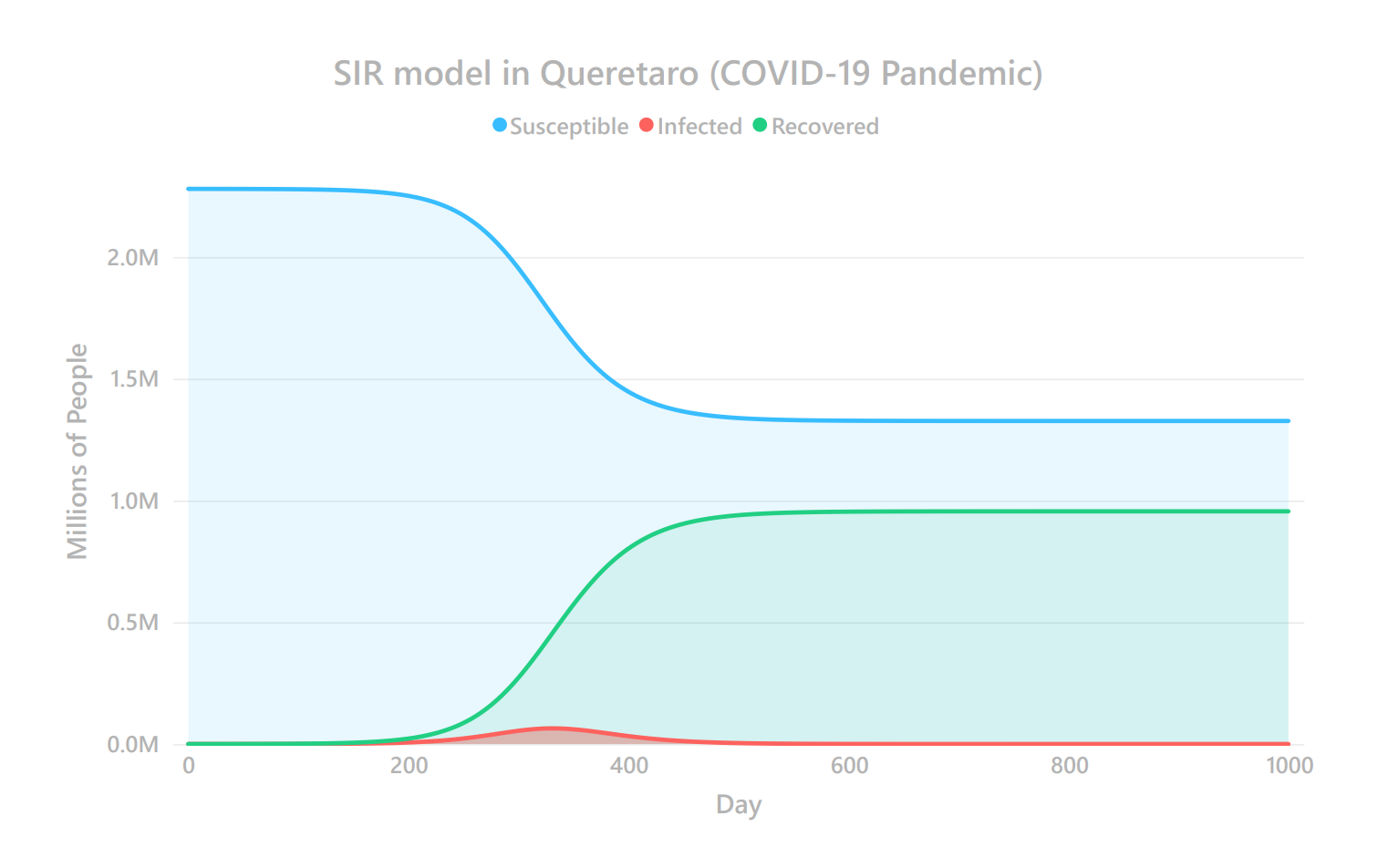
After defining the SIR model functions in Python, as well as the RK4 method, the following forecast was obtained:

In this graph, the blue line represents susceptible people, the green line represents recovered people, and the red line represents people infected with the virus.
- We can see that a “bottleneck” is formed with susceptible and recovered people. This indicates that not all people will get sick from COVID-19 in the State of Queretaro.
- We see that the red line forms a crest, whose highest point represents the maximum number of infected people.
- The horizontal axis represents the day from the initial date of the study (April 6, 2020).
In detail,
+64K
maximum number of infected people
3/03/2021
date of maximum infected people
14.4%
of those infected will die as a result of the virus.
58.19%
percentage of the population that will never contract COVID-19.
Recommendations to Improve the Forecast
- Recalculating beta and gamma with recent dates: As noted, the SIR model depends on the accuracy of the calculation of the beta and gamma factors. Since we started calculating them in April (first cases of Covid in Queretaro), this could have introduced a lot of noise into the final values, since the number of infected and recovered cases at that time was small, and the finite difference method would not be very precise.
To avoid this, it is proposed to take a date range from July 27 to October 27, 2020. This would reduce the standard deviation in the values, and would better fit a scenario where safety and hygiene measures have been taken (such as isolation, the use of face masks, and social distancing).
Acknowledgment
I would like to thank Dr. U. Velasco for encouraging the participation of students (including myself) in using mathematics for real-world applications, and for supporting me at every stage of this study project. I would also like to thank my friend, B. Salgado, for helping me understand the SIR model and its numerical solutions.
References
Show References
- Brauer, F., Castillo-Chávez, C., De La Pava, E., Castillo-Garsow, C., Chowell, D., Espinoza, B., & Moreno, V. (2015). Modelos de la propagación de enfermedades infecciosas. Universidad Autónoma de Occidente.
- Gobierno del Estado de Querétaro. (2020). Datos Estatales de Pandemia por COVID-19. 2020, de Gobierno del Estado de Querétaro. Website: Archive
- Zill, D. G., Hernández, A. E. G., & López, E. F. (2009). Ecuaciones diferenciales con aplicaciones de modelado. México: Cengage Learning.
- Cervantes, F. (2005). Metodo de Diferencias Finitas. México. Instituto Politécnico Nacional. Website: IPN.