Forecasting Sales From a Limited-Time Offer on HumbleBundle
Summary
Machine learning tools were used to make a sales projection (power series regression) for a 3D asset pack that was on sale for 20 days on Humble Bundle. The number of copies sold was 10.49% above the estimated sales.

Date
- Data Science
Category
Python, Power BI
Tools
A New Business Approach
Launched in 2010, Humble Bundle sells games, e-books, software, and other digital content.
With each type of product they sell, a portion of the proceeds is contributed to charitable organizations. For many products, the user can allocate a portion (or even the entirety) of their purchase to the charity of their choice.

This year, I will participate in a bundle on the platform, offering a 3D vehicle pack. My goal in this project will be to forecast how many units of this bundle will be sold in order to estimate revenue (this data won’t be shared).
Problem
- I want to know how many units will be sold by the end of the bundle offer to estimate the earnings.
Solution
- Use regression techniques to find a function that describes the behavior of the data, allowing for an estimate of the final sales.
The offer for this bundle will run from September 26th to October 16th, with the possibility of extending it for approximately 2 more weeks; however, this is not guaranteed. Because of this, the forecast will cover only up to October 16th.


Workflow
The development of this project was divided into 5 phases:
Theoretical Framework
First, a study was conducted on the mathematical justification of regression algorithms and transformations to linearize non-linear relationships.
Linear Regression
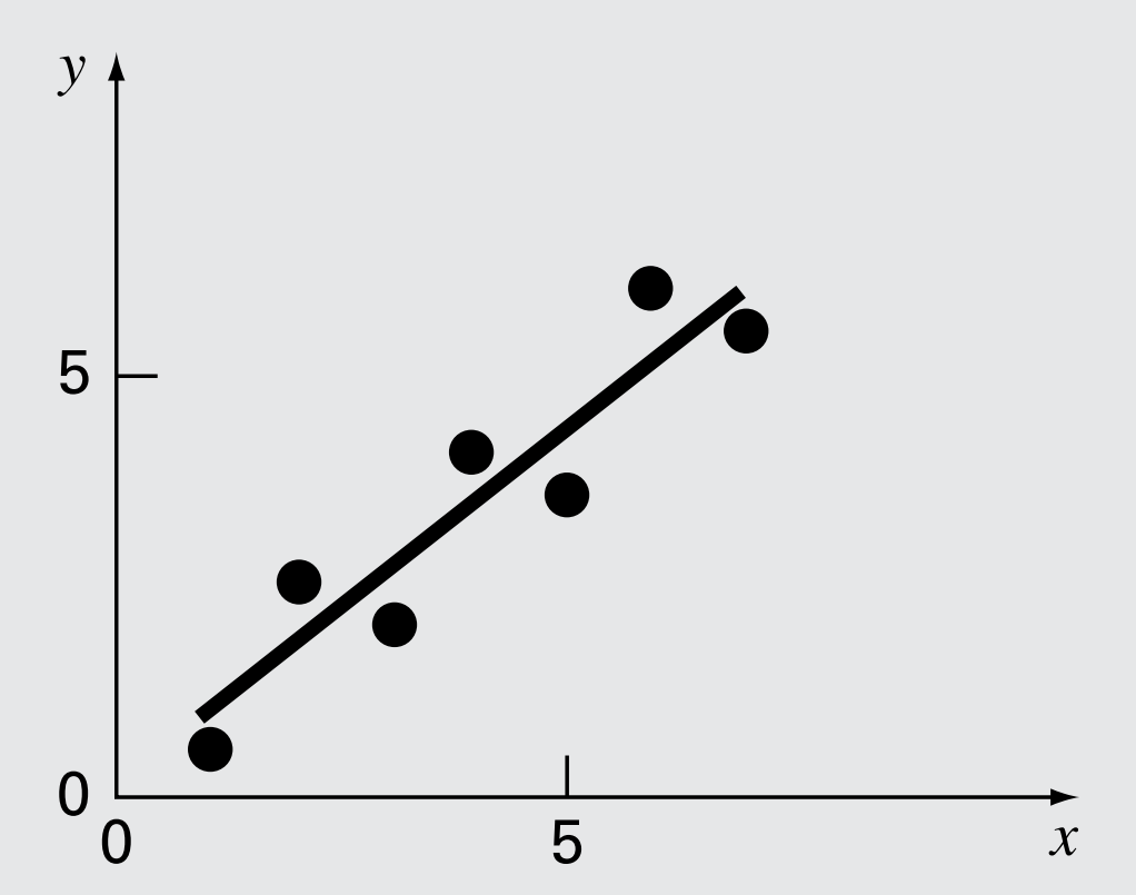
Linear regression is a statistical method that seeks to find the linear relationship between a dependent variable and one or more independent variables through mathematical functions, minimizing the errors between the observed and predicted values.

Function that describes the behavior of the data through linear regression.
The simplest case of least squares regression is fitting a straight line to a dataset, which is mathematically represented as:
[math]y=a +b\cdot x+e[/math]
where a and b are coefficients representing the y-intercept and the slope, respectively, and e is the error, or difference, between the model and the observations.
From this model, different criteria can be derived to reduce the error between the line and the observations. However, the most useful one is the one that minimizes the sum of the squared residual errors, which is mathematically represented as:
[math]S_r=\sum_{i=1}^ne_i^2=\sum_{i=1}^n(y_i-a-b\cdot x_i)^2[/math]
Where yi and xi are the values from the dataset.
Now, to determine the coefficients a and b. We differentiate with respect to each of them:
[math]\frac{\partial S_r}{\partial a}=-2\sum (y_i-a-b\cdot x_i)[/math]
[math]\frac{\partial S_r}{\partial b}=-2\sum x_i(y_i-a-b\cdot x_i)[/math]
The minimum of the sum is found by setting both partial derivatives to 0. By applying some properties of the sums, we obtain the system of equations:
[math]a n+b \sum x_i=\sum y_i[/math]
[math]a\sum x_i+ b\sum x_i^2=\sum x_iy_i[/math]
These are known as the normal equations, and by solving them for the coefficients, we obtain the equation of the line that minimizes the square of the vertical distance between the estimated line and the points.
Linearization of a Power Equation
Linear regression provides a powerful technique for fitting the best line to the data. However, it assumes that the relationship between the dependent and independent variables is linear. In some cases where this condition is not met, transformations can be used to express the data in a form compatible with linear regression.
For example, we can linearize a power series model as follows:
[math]y = a \cdot x^b[/math]
[math]\log(y) = \log(a \cdot x^b)[/math]
[math]\log(y) = \log(a) + b \cdot \log(x)[/math]
In this way, a plot of log (y) against log (x) will result in a straight line with slope b and an intercept on the ordinate axis of log(a). Since the relationship between x and y is now linear, we can apply the least squares regression algorithm to determine a and b.
Finally, we apply another transformation to return to the original relationship (power series) and use the obtained values of a and b in the regression model.
[math]10^{\log(y)} = 10^{\log(a) + b \cdot \log(x)}[/math]
[math] y = 10^{\log(a)} \cdot 10^{b \cdot \log(x)}[/math]
[math]y= a \cdot x^b[/math]
This is the linear regression chosen for this project (based on the behavior of the data).
Ask
Then, Business Task was defined, as well as a series of questions that guided the forecast.
Show Guiding Questions
- How many data records are enough to make a reliable projection?
- What kind of behavior does the cumulative sales data have?
- What type of function best resembles the behavior of the data (logarithmic, polynomial, etc.)? Why?
- Are there external factors that affect total sales (marketing campaigns, day of the week, time remaining)?
Business Task
Use the sales data from the first 5 days of the 3D package with regression techniques to find a function that describes its behavior, allowing us to estimate total sales.
Prepare
Data sources were defined, their credibility was confirmed, and issues with bias, privacy, and accessibility were identified.
Where is the data stored?
The data was collected manually from the Humble Bundle website.
How was the data collected?
Data on copies sold and average purchase price was recorded daily at 12:00 p.m. (GMT-6) from September 27, 2024, to October 16, 2024, on the Humble Bundle website.
How is the data organized?
It is organized in long format.
It includes data on: day number, date, total sales and sales per day.
Are there issues with credibility in this data?
There are no issues with the credibility of the data, as it was collected directly from the HB website. Additionally, I set an alarm each day at 12:00 p.m. to remind myself to collect the data; I didn’t miss a single day.
How am I addressing licensing, privacy, security, and accessibility?
Since no individual’s name is mentioned and the data is public, there are no privacy, confidentiality or licensing issues with the use of this data sets.
Process
Software tools were defined.
- Data sets were organized and cleaned (using Excel).
- Regression model of power series was made (using Python).
Show Data Processing (Excel)
Every day at 12:00, I visited the HumbleBundle website to check how many cumulative sales the bundle had. I saved this data in an Excel file (date, number of sales, and their logarithmic values, which were used in the regression model).

Show Regression Model (Python)
Implementing linear regression (least squares) was relatively straightforward since the mathematical expressions are quite clear.
You can find the complete Python code below. It returns the values for the coefficients a and b, which will be used in the power series model.
As I mentioned, I used data from the first 5 days of the special sale to create this model. Additionally, I calculated the base-10 logarithms of these values because I linearized a power equation.
					import math

# Log10 values of day (xi) and sales (yi)
xi = [0.0, 0.301029, 0.477121, 0.602059, 0.69897]
yi = [2.863322, 3.013258, 3.085647, 3.142702, 3.18949]

# Regression variables
sum_xiyi = 0.0
sum_xi = 0.0
sum_xi2 = 0.0
sum_yi = 0.0
average_x = 0.0
average_y = 0.0
a = 0.0
b = 0.0

def solve_least_squares():
    global sum_xiyi, sum_xi, sum_xi2, sum_yi, average_x, average_y, a, b

    # Enfoque: y = b + a * x + e
    n = len(xi)
    for i in range(n):
        sum_xiyi += xi[i] * yi[i]
        sum_xi += xi[i]
        sum_xi2 += xi[i] ** 2
        sum_yi += yi[i]

        if i == (n - 1):
            average_x = sum_xi / n
            average_y = sum_yi / n

    b = ((n * sum_xiyi) - (sum_xi * sum_yi)) / ((n * sum_xi2) - (sum_xi ** 2))
    a = average_y - (b * average_x)

    print(f"Linear Regression: y = {a} + {b}x")

solve_least_squares()
Analyze
The data was analyzed using Power BI.
Insights are explained in detail in the following section, “Forecast”.
Forecast
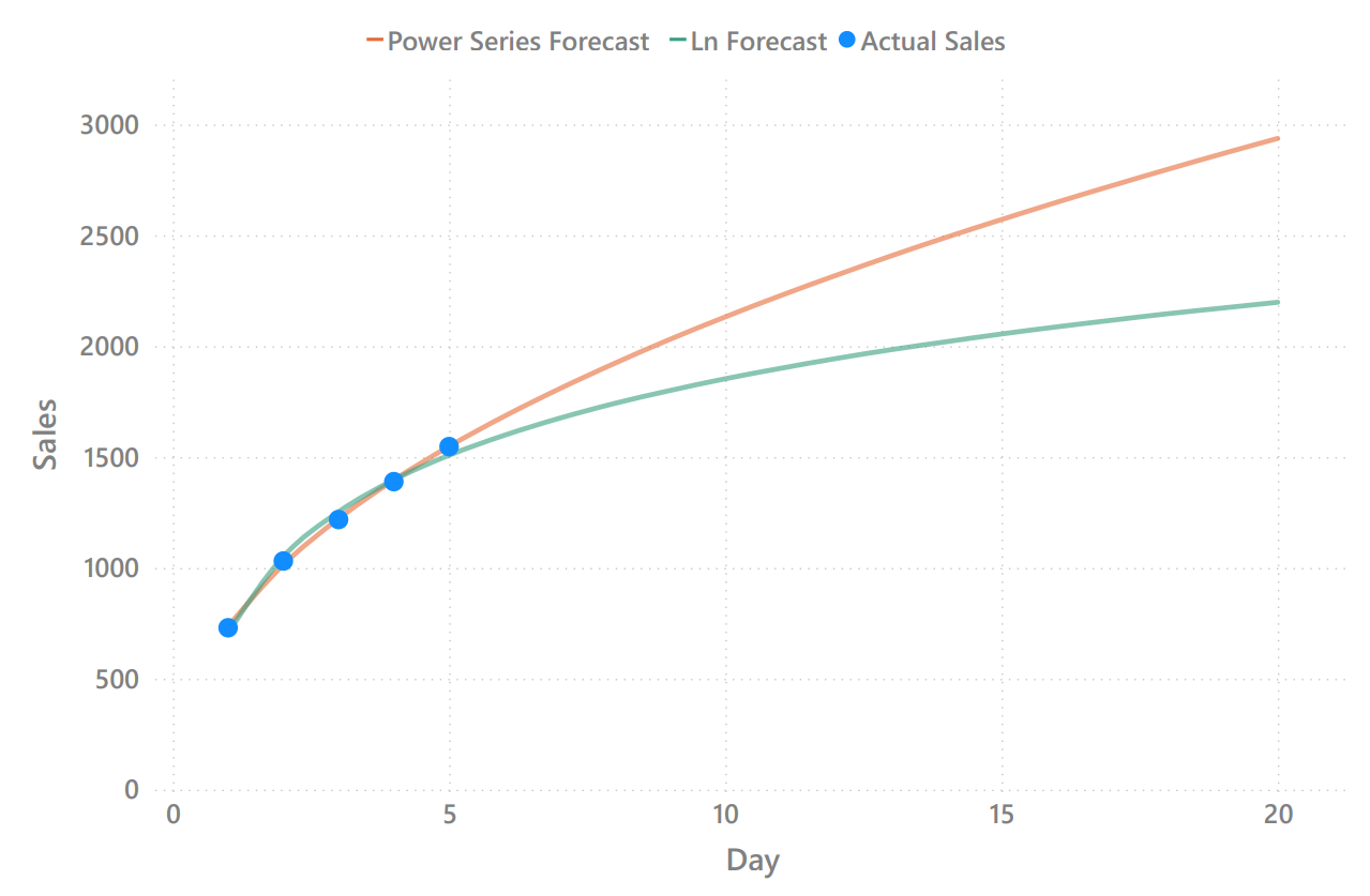
I considered two types of mathematical functions that could best describe the data’s behavior: power series (orange line) and logarithmic (green line) functions.
Ultimately, I chose the power series model because it resulted in a lower mean squared error compared to the logarithmic model.
Two Regression Models: Power Series & Natural Logarithm

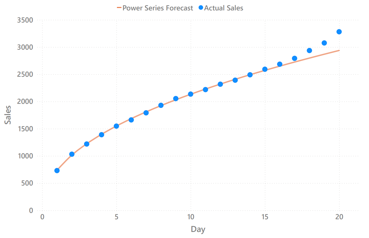
With this regression, I estimate that sales will reach approximately 2,940 units by the end of the bundle offer (on October 16, 2024).
After this 20-day period, this was the performance of my forecast.
Comparison of Total Sales & Regression Model

2937
units (projected sales)
3281
units (actual sales)
+10.49%
There were 10.49% more units sold than projected
Understanding Sales Increment
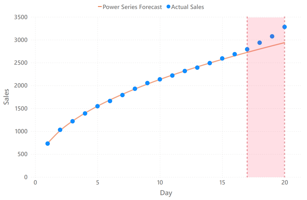
As we can see, the model described the sales quite well during most of the bundle offer, but something happened during the last 4 days of the sale: there was an increase in units sold.

Since there were no marketing campaigns or social media posts promoting this bundle, I infer that this increase was driven by FOMO (Fear of Missing Out) factors on the HumbleBundle website.
According to Intuit Mailchimp: “FOMO marketing uses psychology to tap into consumers’ emotional responses and triggers, making them want to act quickly to avoid missing out on an opportunity.”
So, what changed during the last 4 days of the sale? Check these pictures:


These were the cards listed in the HB store.
The difference is that in the second one (used during the last 4 days of the sale), there is a red sign serving as a clear ‘call to action’ button. Additionally, instead of only displaying the days remaining, it also includes hours, minutes, and seconds.
This may seem like a subtle change, but it emphasizes the limited availability of the offer. This can accelerate the decision-making process and encourage customers to commit (Intuit Mailchimp).
Update: The offer has been extended until November 3rd
Initially, this bundle was going to be available only for 20 days, starting on 26/sep and ending on 16/oct. However, it was extended to 3/nov.
This increased the number of copies sold from 3281 to 4785! Also, there were 2 more FOMO events within the HumbleBundle website.
Despite this, it was not certain that the sale would be extended until November 3rd, so the model was adjusted to describe the data only up to October 16th.
References
Show References
- Chapra, S.C., Canale, R.P., Ruiz, R.S.G., V.H.I., Díaz, E. M., & Benites, G. E. (2015). Métodos numéricos para ingenieros (Vol. 7). México: McGraw-Hill.